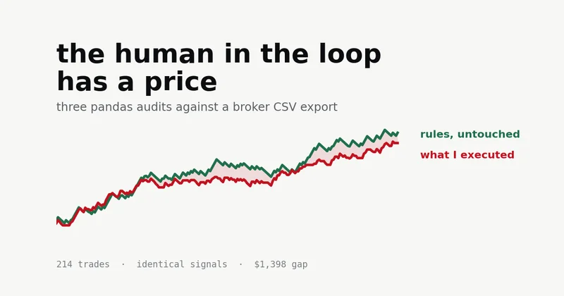
Every automated system that still has a human with override permissions is not an automated system. It is a hybrid, and the human half never gets profiled.

I spent years shipping trading rules I described as systematic. Entry conditions in code, stop distance in code, position size in code. And then, most days, I would do something slightly different from what the code said, because I was watching, and watching produces opinions. Skip the setup that looks weak. Flatten before the news. Take the profit early because giving it back would feel worse than never having it.

None of that shows up in a trade log. A trade log records what happened. It does not record what would have happened, so the gap between the two is invisible by construction. That gap is the thing I wanted a number for.

It turns out you can get one with about eighty lines of pandas against a broker CSV export. Below are three audits I run monthly, the code for each, and what they returned on a sample log. Every figure in this article comes from a synthetic 214-trade dataset built for the walkthrough, not from anyone's live account, so treat the numbers as a worked example rather than a claim about markets.

The Setup

You need two things joined on a trade ID: what you did, and what the rules said to do. Most brokers export the first. The second you have to reconstruct, either from your strategy's own signal log or by replaying the rules over the same bars.

The sample log has 214 trades over roughly six months. The underlying system risks a fixed dollar amount per trade, stops out at -1R, targets +2R, and produces +0.29R per trade on a 44% win rate when left alone. The human layer on top skips roughly one signal in ten, cuts winners early about a third of the time, moves the stop to breakeven once a trade is comfortably green, and occasionally sizes up after a loss.

Those four behaviors are the entire difference between the two curves below, and my prior going in was that they would all be expensive. That prior was wrong in a way I found more useful than being right.

Audit 1: The Intervention Tax

The headline number is a subtraction. Same signals, same bars, one curve where the rules ran untouched and one where I was in the loop.

```
import pandas as pd
df = pd.read_csv("trade_log.csv") # trade_id, sys_pnl, act_pnl, behaviour
tax = df.act_pnl.sum() - df.sys_pnl.sum()
print(f"system: ${df.sys_pnl.sum():,.0f}")
print(f"actual: ${df.act_pnl.sum():,.0f}")
print(f"tax: ${tax:,.0f} ({tax / df.sys_pnl.sum():.0%} of gross)")

same subtraction, split by what I did

by_habit = (df.assign(delta=df.act_pnl - df.sys_pnl)
.groupby("behaviour")["delta"]
.agg(["count", "sum"])
.sort_values("sum"))
print(by_habit)
```

On the sample log, the system produced $12,337, and the executed version produced $10,939. The tax is $1,398, about 11% of gross.

Eleven percent is not a catastrophe, which is exactly why nobody catches it. It does not read as a leak. It reads as a slightly disappointing six months, and the natural response to a slightly disappointing six months is to go looking for a better strategy.

The breakdown is where it gets useful:

| habit | trades | delta |
|---|---|---|
| cut winners early | 26 | -$2,161 |
| skipped signals | 24 | -$423 |
| moved stop to breakeven | 38 | -$22 |
| sized up after a loss | 49 | +$662 |

One habit accounts for more than the entire tax. Cutting winners early cost more than the net gap, and the other three partly offset it. Of the 26 trades I cut at +0.8R, 19 went on to hit the +2R target under the rules. The others would have come back and stopped out, which is the memory that makes the habit feel justified.

The breakeven column is the one that surprised me. It is the single most argued-about habit in retail trading, and in this sample, it was worth negative twenty-two dollars across 38 trades. Not good, not bad, noise. I had assumed for years it was either saving me or killing me, and it turned out to be neither, which meant every hour I had spent thinking about it was an hour not spent on the exit rule that was actually bleeding.

Sizing up after a loss made $662, and this is the trap the audit is designed to catch rather than endorse. That habit does not have positive expected value. It multiplies the size of whatever comes next, and across 49 trades the coin landed favorably. Judging a variance-increasing habit by its realised P&L over 49 samples is exactly the reasoning error the script exists to replace. The right column to look at there is not the sum; it is the worst drawdown with and without.

Audit 2: Stop distance against your own MAE.

The second audit asks whether a parameter you set once, probably with a round number, matches the data you have since collected.

Maximum adverse excursion is how far a trade went against you before it did whatever it did next. Most platforms export it. If yours does not, join entry and exit timestamps to 1-minute bars and take the extreme in that window. Slightly overstates heat on long holds, close enough to size from.

w = df[df.sys_R > 0] l = df[df.sys_R < 0] print(f"winners: median MAE {w.mae_R.median():.2f}R, " f"25th pct {w.mae_R.quantile(.25):.2f}R, " f"share past -0.70R {(w.mae_R <= -0.70).mean():.0%}") print(f"losers: median MAE {l.mae_R.median():.2f}R") ax = l.mae_R.plot.hist(bins=20, alpha=.55, label="losers") w.mae_R.plot.hist(bins=20, alpha=.75, ax=ax, label="winners") ax.axvline(-1.0, ls="--", color="k") # where the stop actually sits ax.legend()

In the sample, winners had a median MAE of -0.29R and 18% of them dipped past -0.70R before working. The stop sits at -1.0R, so it is outside the range where most winners breathe, but not by a lot, and the tail of the winning distribution runs right up to it.

That tells you the stop is defensible. It does not tell you it is optimal, and the histogram alone cannot, because moving the stop changes the size you can carry at constant dollar risk. The sweep does:

def replay(path, stop, target=2.0): """Re-run one trade's price path against a different stop. R is normalised so dollar risk per trade stays constant.""" for x in path: if x <= -stop: return -1.0 if x >= target: return target / stop return path[-1] / stop for s in [0.70, 0.85, 1.00, 1.20, 1.50]: res = np.array([replay(p, s) for p in paths]) print(f"stop {s:.2f}R -> win rate {(res>0).mean():.0%}, " f"expectancy {res.mean():+.3f}R")
| stop | win rate | expectancy |
|---|---|---|
| 0.70R | 36% | +0.364R |
| 0.85R | 42% | +0.367R |
| 1.00R | 44% | +0.288R |
| 1.20R | 44% | +0.206R |
| 1.50R | 44% | +0.164R |

Tighter was better in this sample, and the win rate went the other way. Between a 0.85R and a 1.5R stop, the win rate is flat or improving while expectancy halves, which means win rate carried no information about the parameter at all. If you are tuning a stop by watching how often you get stopped out, you are optimising a metric that is disconnected from the outcome you care about.

I am not claiming tighter stops are generally better. This is one synthetic dataset with a target fixed in absolute terms, and that assumption is doing real work in the result. The transferable part is the method: replay your own paths, sweep the parameter, look at expectancy rather than hit rate, and find out whether the number you have been using since you started was ever tested.

Audit 3: The counterfactual on a single habit.

The third audit isolates one behaviour and asks what the alternative would have paid. Breakeven is the natural candidate because it is a discrete, taggable event.

be = df[df.behaviour.str.contains("be_stopped")] print(f"trades where I moved to BE: {len(be)}") print(f"actually collected: ${be.act_pnl.sum():,.0f}") print(f"rules would have: ${be.sys_pnl.sum():,.0f}") print(f"of those, would have won {(be.sys_R > 0).sum()}, " f"lost {(be.sys_R < 0).sum()}")

Thirty-eight trades, $0 collected, $22 under the rules. Fourteen of them would have been winners I gave up; 24 would have been losses I avoided. The habit is a wash in dollars and a meaningful reduction in variance, which is a defensible thing to want and a completely different justification from the one I had been using. I thought breakeven was making me money. It was buying me smoothness, at roughly cost, and I should have been deciding whether smoothness was worth that price rather than assuming it was free.

Run the same template on any habit you can tag: the news filter, the Friday skip, the rule about not trading after two losses. The pattern is always the same three lines. What did I collect, what would the rules have collected, and how does the split between avoided losses and forfeited wins actually look?

What the audit is really for

None of this makes you follow your rules. Knowing the number is not the same as behaving differently, and I have the six months of logs to prove it.

What changed things for me was moving the decisions that survived the audit into code where I could not reach them, and leaving the rest as explicit, logged overrides. Not because judgment is worthless, but because judgment at 09:40 with a position open is a different function than judgment on a Sunday with nothing at stake, and only one of those has time to think. The intervention tax is the price difference between the two functions, and it is measurable to the dollar.

There is a second-order lesson that took me longer. When I first tried to log heat live, marking each trade as it went against me, the act of logging changed how long I held. The measurement modified the thing being measured, and afterwards there was no way to separate the two columns. Everything here runs after the close, off exported data, with no human in the measurement loop either.

If you run any system with a manual override, the audit is a weekend of work, and it gives you a number you have almost certainly never seen. It might be small. Mine was 11%, which was small enough to ignore and large enough to matter, and the distribution across habits was nothing like what I would have guessed.

If you cannot remove the human, at least meter them.

Mateo Rivera builds systematic trading strategies at Puravida Edge.