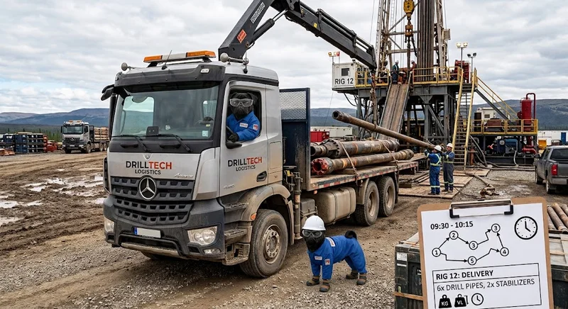
Words that make your shoulders tense the moment you hear them. Words that create that strange void in your stomach, like when an elevator drops a little too fast.

Got them?

For me, those words were:

Los Movimientos — “The movements,” in English.

Back when I worked in oil and gas, my colleagues Jesús B, Karina G. and I were responsible for planning and coordinating every movement of tools and personnel required by the drilling operations across eastern Venezuela for a major oilfield services company.

And when activity was at its peak, there were a lot of movements.

We were supporting around 50 drilling jobs per month. On any given day, roughly a dozen heavy trucks might be dispatched to deliver or collect drilling tools, while another dozen light pickup trucks transported directional-drilling crews between operational bases, hotels, and active drilling rigs.

Most movements involved delivering something from the operational base to a rig, or bringing tools and personnel back from the field. But sometimes we also had lateral movements between rigs: collect a tool from Rig A, deliver it to Rig B, pick up a crew somewhere else, and somehow get everyone where they needed to be before the driving restrictions kicked in.

Every afternoon, usually around 4 p.m., the requests started arriving.

Not one by one, calmly and politely.

They arrived as a flock.

Field service managers would send the required tool movements, personnel movements, urgent pickups, rig-to-rig transfers, and last-minute changes. From that pile of requests, I had to construct the route of every truck and every pickup for the following day.

And the vehicles did not necessarily begin at the operational base. Their starting locations depended on where they had finished the previous day. A truck might be parked at the base, at a rig, or somewhere else entirely. The same was true for the crews.

To make things more entertaining, driving after 8 p.m. was forbidden except under exceptional circumstances.

And no, this was not some annoying bureaucratic rule invented to make our lives more difficult. We were constantly reminded that road accidents were among the greatest dangers in oilfield operations. Moving people and heavy equipment across long distances, often on poor roads and after exhausting shifts, was serious business.

So every route had to work.

The vehicle needed enough capacity. It had to begin in the correct location. It had to collect each item before delivering it. The crew needed to be picked up before they could be dropped off. The truck had to reach each rig at a reasonable time. And everything had to finish before the evening driving restriction.

Let me tell you: this task was soul-crushing.

Planning each truck felt like solving a horrible maze combined with a difficult Sudoku puzzle, except the Sudoku puzzle could call you the next morning and tell you that you had f*cked it up.

I could easily spend several hours every afternoon planning the routes. I did it with pen and paper.

Well, pen, paper, and an Excel spreadsheet.

But Excel was not helping much.

I would eventually finish, look at the plan, and convince myself that everything made sense. Then, the following morning, I would discover that one route was infeasible, that a tool could not arrive on time, that a vehicle had been assigned somewhere else, or that a sequence I had proposed simply did not work.

Then everything had to change again.

It was deeply demoralizing.

Perhaps you have experienced something similar. There is a particular kind of frustration that comes from not knowing how to do your job well and, even worse, having absolutely no idea how to improve.

You know there must be a better way. You suspect that someone, somewhere, has already solved a similar problem. But you do not even know what words to type into Google.

That was exactly where I was.

This was 2015–2016. There was no ChatGPT, no Claude, and no helpful chatbot waiting to explain vehicle-routing models to an exhausted drilling engineer at five in the afternoon.

I searched online for things like “transportation planning,” “truck routing,” and “logistics optimization.”

What did I find?

Mostly advertisements from trucking companies and generic logistics blogs explaining that transportation was important.

Thank you. Very helpful.

The only genuinely useful thing Jesús and I found was an article saying that we needed to construct a distance matrix. So we began doing exactly that.

Jesús, Karina, we were on the right track.

But, analytically speaking, we were also so incredibly far away.

It was like going to a doctor knowing that you were sick, but not knowing what disease you had, what kind of specialist you needed, or even how to describe the symptoms.

Where do you begin when you do not know the name of the problem?

The worst part was that, from the outside, none of this looked particularly difficult.

Other people would casually assume that planning the movements should be easy. Just assign a few trucks, draw some routes, and send them out.

But I have not yet told you the most painful part.

We did not have a dedicated fleet.

The heavy trucks and pickups came from a shared pool used by several oilfield service segments. My segment was drilling, but other business lines were competing for the same vehicles. If one truck was assigned to us, that was one truck unavailable to another operation.

So we were not merely trying to design good routes.

We were trying to design them with scarce resources, under time restrictions, with uncertain starting locations, paired pickup-and-delivery requirements, vehicle-capacity limits, and constant competition for the fleet.

It felt like fighting a battle that had already been lost.

Today, after completing a PhD in economics and spending most of my research life working in operations research, I finally know what kind of monster we were fighting.

And let me tell you, it was a tough motherf*cker.

So, Jesús and Karina if you are reading this: we had no chance.

We did the best we could with the tools and knowledge we had. Honestly, it is kind of miraculous that we managed to keep the entire operation running that way.

The monster even has one of those absurdly long names that sounds like the title of a medieval king:

The Capacitated Pickup and Delivery Vehicle Routing Problem with Time Windows

How the f*ck were we supposed to search for that in 2015?

And even if, through some miracle, we had discovered the correct name, have you seen the mathematical formulation of this thing?

Do not worry. You will see it in the next sections.

But if I had encountered those equations back then, without my current training, I would have assumed they were arcane magic. Strange runes written by some secret society of mathematicians who had never experienced the joy of receiving twelve urgent transportation requests at 4:45 p.m.

The formulation looks awful.

It looks dense, intimidating, and almost deliberately indigestible.

But the underlying logic is not magic. It is simply a precise way of describing the same nightmare Jesús and I were trying to solve every afternoon with paper, intuition, and a barely useful Excel sheet.

That is why I am writing this article.

Perhaps you are currently in the same position I was in. Perhaps you are planning deliveries, collections, service visits, technicians, medical transportation, warehouse transfers, or field crews. Perhaps you know your current process is inefficient, but you do not know what the problem is called or where to start.

I do not want you to struggle with it without knowing what you are dealing with.

I see this article as a gift to my previous self: the explanation and working example I desperately needed back then.

And if one of my former colleagues who is still working in oil and gas happens to read this, especially now that there is renewed talk of increasing drilling activity in Venezuela, please:

Try planning Los Movimientos this way.

It will help. A lot.

In this article, we will:

Translate the real-world nightmare of Los Movimientosinto a formal pickup-and-delivery routing problem.
Understand the main elements of the problem, including vehicles, pickup locations, delivery locations, capacities, travel times, and time windows.
Build a small but realistic example that captures the essential difficulties of the original operation.
Formulate the problem as a mixed-integer linear programming model.
Explain each decision variable, constraint, and objective-function term in plain language.
Implement the complete model in Python using Pyomo.
Solve the model with the open-source HiGHSoptimizer.
Extract the optimized vehicle routes from the solution.
Visualize the resulting pickup-and-delivery plan.
Discuss the limitations of the model and how it could be extended to larger and more realistic operations.

By the end, you will have a complete working example that you can adapt to your own transportation, field-service, or last-mile delivery problem.

The Problem: When Every Delivery Also Comes with a Pickup

At first glance, a delivery problem sounds simple.

A customer places an order, a vehicle leaves the depot, delivers the product, and moves on to the next customer.

But many real transportation operations are not that simple.

Sometimes, the vehicle must not only deliver something, but also pick something up.

This is extremely common in modern retail, e-commerce, and last-mile logistics.

Consider grocery delivery services that use reusable containers. A driver may deliver milk, juice, or other products in returnable bottles or crates, while collecting the empty containers from a previous order.

The same logic appears in furniture and household-appliance delivery. A company may deliver a new refrigerator, washing machine, sofa, or mattress while also collecting the customer’s old one. In some countries, including France, this type of take-back service is common and may even be required in certain situations.

The vehicle therefore performs two connected operations:

Pick up an item at one location.
Deliver that same item to another location.

Sometimes the direction is reversed from what we usually imagine. The vehicle delivers a new product to the customer and then collects an old product that must be transported back to a warehouse, recycling center, or disposal facility.

These paired operations create what is known as a pickup-and-delivery request.

The key word here is paired.

If a vehicle collects an item, that same item must eventually be delivered somewhere. More importantly, the pickup must happen before the delivery.

You cannot deliver a refrigerator that you have not yet collected.

You cannot drop off a drilling tool at a rig if the truck has not first picked it up from the operational base.

You cannot return an empty bottle to the distribution center if the driver has not yet visited the customer.

This creates a precedence relationship between the two locations.

And that is only the beginning.

Time windows make everything harder

Customers are not always available throughout the entire day.

A household may request delivery between 8 a.m. and noon. A store may only accept deliveries before opening hours. A warehouse may stop receiving trucks after 4 p.m. A drilling rig may require a tool before the start of a critical operation.

These restrictions are represented using time windows.

For each pickup or delivery location, we define an interval:

where:

is the earliest time service can begin;
is the latest time service can begin.

A vehicle may arrive early, but it must wait until the time window opens. If it arrives after the closing time, the visit is no longer feasible.

Time windows may arise for several reasons.

Some are customer-related. A customer may only be available during a specific period.

Others come from operational restrictions. Warehouses, stores, construction sites, hospitals, and industrial facilities may only receive vehicles during certain hours.

Cities may also restrict the circulation of heavy vehicles during parts of the day. A truck may be allowed to enter a neighborhood only in the morning, or it may be forbidden from circulating during peak traffic hours.

Companies may also operate under service-level agreements. A same-day order may need to be delivered within six hours. A medical sample may need to reach a laboratory before a deadline. A spare part may need to arrive before a maintenance team can begin its work.

In the case of Los Movimientos, the time restriction was particularly strict: vehicles were generally not allowed to drive after 8 p.m or before 6 a.m. Every route therefore had to be completed within that window.

Capacity matters too

Vehicles cannot carry an unlimited amount of goods.

A small pickup truck may transport a few boxes or a crew of workers. A heavy truck may carry several large drilling tools, but even that truck has a maximum capacity.

This means that the order of the visits matters.

Suppose a vehicle has capacity for ten units. It cannot pick up three orders of five units each before delivering any of them. At some point, it would be carrying fifteen units, which is impossible.

The route must therefore be designed so that the vehicle load never exceeds its capacity.

Pickups increase the load of the vehicle.

Deliveries decrease it.

This creates another dynamic element: the amount carried by the vehicle changes continuously along the route.

Not every vehicle can serve every request

Real fleets are rarely perfectly homogeneous.

Some requests require refrigerated vehicles. Others require trucks with lifting equipment, enough cargo space, specific permits, or drivers with particular qualifications.

In oilfield operations, certain tools could only be transported by particular types of trucks. Personnel movements required light pickups, while heavy equipment required larger vehicles.

The model must therefore account for compatibility.

A request may be assigned only to a vehicle that is physically and operationally capable of performing it.

Vehicles may start in different places

Many textbook routing problems assume that every vehicle begins and ends at the same depot.

Reality is often messier.

A truck may begin the day at the operational base. Another may have spent the night at a drilling rig. A third may start at a maintenance facility after being repaired.

The same vehicle may also finish the day somewhere different from where it started.

This matters because the starting position of a vehicle determines which requests it can serve efficiently.

A truck already located near a pickup point may be a better choice than one that must travel two hours before beginning the route.

Sometimes there are not enough vehicles

This is where the problem becomes especially painful.

The company may receive more transportation requests than the available fleet can handle.

Some requests may then have to be postponed, outsourced, or left unserved.

In the formulation we will use, unserved requests are placed in what the original authors call a request bank. The optimization model applies a large penalty to each request left there, encouraging the solver to serve as many requests as possible.

This is useful because it prevents the entire model from becoming infeasible when the available vehicles are insufficient.

Instead of simply declaring, “No solution exists,” the model tells us:

This is the best plan possible with the vehicles currently available, but these requests cannot be served.

That is an important distinction in practice.

The Model

So what exactly are we trying to decide? Given:

a set of pickup-and-delivery requests;
a fleet of vehicles;
vehicle capacities;
travel times and distances;
time windows;
vehicle-request compatibility;
starting and ending locations;
and possibly too few vehicles;

we must determine:

which vehicle serves each request;
the order in which each vehicle visits its locations;
when service begins at every location;
how the vehicle load changes along the route;
and which requests, if any, must remain unserved.

The goal is to construct routes that are feasible while minimizing a combination of:

total distance travelled;
total operating time;
and the number of unserved requests.

This is the Capacitated Pickup and Delivery Problem with Time Windows.

And now that the monster has a name, we can finally begin describing it mathematically. We are going to use the formulation described by Psinger et al. 2006 [1] that the authors describe as the PDPTW.

At first glance, the formulation looks intimidating, but the logic is actually quite natural. The model is simply trying to answer a practical question:

Which vehicle should do which pickup-and-delivery jobs, in what order, at what time, and without violating capacity or timing restrictions?

The model does this by choosing vehicle routes while minimizing total transportation cost.

The objective function at the top minimizes three things at once:

Total distance traveledby all vehicles.
Total time spent by the vehicleson their routes.
The number of requests left unserved.

That third term is important. If there are not enough vehicles or the requests are too difficult to schedule, the model is allowed to leave some requests out, but it pays a penalty for doing so. In practice, this penalty is usually set high so that the model tries very hard to serve everything.

Before looking at the constraints, it helps to understand the variables.

xtells us whether a vehicle goes directly from one location to another.
In plain English, this variable builds the actual route.
Stells us the time at which a vehicle starts service at a location.
This is how the model keeps track of timing.
Ltells us the load of the vehicle after servicing a location.
This is how the model keeps track of capacity.
ztells us whether a request is left unserved.
If it is, that request goes into the request bank.

Constraint (1): every request must be handled somehow

Constraint (1) says that each request must have exactly one outcome:

either it is assigned to a compatible vehicle,
or it is left unserved.

So the model cannot accidentally forget a request, and it cannot assign the same request to multiple vehicles.

Constraint (2): pickup and delivery must be done by the same vehicle

Constraint (2) ensures that if a vehicle performs the pickup of a request, then that same vehicle must also perform the corresponding delivery.

This is essential. Otherwise, the model could create nonsense solutions where one truck picks up an item and another truck magically delivers it later.

So this constraint keeps the pickup and delivery linked together as one coherent job.

Constraint (3): every vehicle must leave its starting point

Constraint (3) says that each vehicle must depart exactly once from its start terminal.

In practical terms, every vehicle route must begin somewhere specific, such as a depot, a base, or wherever that vehicle is parked at the beginning of the day.

Constraint (4): every vehicle must end at its ending point

Constraint (4) says that each vehicle must arrive exactly once at its end terminal.

So each route has a clear end as well as a clear beginning.

Together, constraints (3) and (4) ensure that every vehicle follows one full route from a start location to an end location.

Constraint (5): route continuity

Constraint (5) is the flow-conservation constraint.

It says that if a vehicle arrives at a pickup or delivery node, it must also leave that node.

This prevents impossible situations where a vehicle:

appears at a location without getting there, or
arrives at a location and then disappears.

This is what makes the chosen arcs form a continuous route rather than a disconnected collection of movements.

Constraint (6): time must move forward along the route

Constraint (6) is one of the most important ones.

It says that if a vehicle goes from location A to location B, then the start of service at B must happen after:

service at A is completed, and
the travel time from A to B has passed.

In everyday terms: a vehicle cannot teleport.

If it loads something at one place, spends some time there, and then drives to the next place, the clock must reflect that.

This constraint also helps eliminate weird circular subroutes, because time must keep moving forward.

Constraint (7): every visit must respect its time window

Constraint (7) enforces the time windows.

Each location has an earliest and latest allowable service time. This constraint ensures that the vehicle starts service within that interval.

This can represent many real-life restrictions, such as:

customer availability,
warehouse opening hours,
delivery deadlines,
circulation restrictions in a city,
or, in my oil-and-gas story, the prohibition on driving too late in the day.

Constraint (8): pickup must happen before delivery

Constraint (8) enforces precedence.

It says that the pickup of a request must happen before the delivery of that same request.

This is a simple idea, but a crucial one.

A truck cannot deliver a tool to a drilling site before it has first collected it.

A delivery crew cannot dispose of an old washing machine before it has first picked it up from the customer.

This constraint enforces that logical order.

Constraint (9): the vehicle load must evolve correctly

Constraint (9) keeps track of the vehicle load from one stop to the next.

When a vehicle visits a pickup location, its load increases.

When it visits a delivery location, its load decreases.

This constraint ensures that the load variable always matches what the vehicle should actually be carrying along the route.

Without this, the model could produce routes that ignore the physical movement of the goods.

Constraint (10): capacity cannot be exceeded

Constraint (10) makes sure that the load of the vehicle always stays between zero and its maximum capacity.

That means:

the vehicle cannot carry more than it is physically able to transport,
and it cannot have a negative load.

So this prevents impossible plans such as loading too much equipment onto one truck.

Constraint (11): vehicles start and end empty

Constraint (11) says that every vehicle begins empty and must also finish empty.

This makes sense in pickup-and-delivery operations, because anything collected during the route is supposed to be delivered somewhere before the route ends.

So the model does not allow a vehicle to finish the day with undelivered goods still on board.

Constraint (12): routing decisions are binary

Constraint (12) says that the routing variable can only take the value 0 or 1.

So for any possible movement, the answer is:

yes, the vehicle uses that arc,
or no, it does not.

There is no halfway value.

Constraint (13): unserved-request decisions are binary

Constraint (13) says that the request-bank variable is also binary.

So each request is either:

unserved,
or not unserved.

Again, there is no in-between.

Constraint (14): time and load cannot be negative

Constraint (14) says that the service times and vehicle loads must be nonnegative. That simply rules out meaningless values like negative time or negative cargo.

The Problem Data

Now that the mathematical monster has been introduced, let us give it something small enough to eat.

The real version of Los Movimientos involved dozens of vehicles, changing starting locations, multiple business units competing for the same fleet, last-minute requests, and enough uncertainty to ruin anyone’s afternoon. Reproducing all of that here would be realistic, but it would also turn this tutorial into another nightmare.

So we will work with a simplified day of personnel transportation.

Our small network contains one operational base and five drilling rigs. Three pickup trucks are available, and each one begins and ends the day at the operational base.

Company policy limits every pickup to four people, including the driver. This means that each vehicle can transport at most three passengers at any given time.

The working day starts at 6:00 a.m. and ends at 8:00 p.m. No vehicle may depart before 6:00 a.m., and every route must be completed by 8:00 p.m. Because the model explicitly tracks travel and service times, it cannot schedule a vehicle to begin a journey that would finish after the cutoff.

We will consider ten transportation requests, each composed of one pickup and one delivery. This gives us twenty service nodes in total.

The requests include the three situations we frequently encountered in the field:

personnel leaving the operational base to begin work at a rig;
personnel being transferred from one rig to another;
personnel finishing their shift and returning to the operational base.

Every group must be collected before it can be delivered, the same pickup truck must perform both parts of the movement, and the truck must never carry more than three passengers.

Each pickup and delivery also has a time window. Some crews need to reach a rig before the beginning of a shift, while others can only be collected after completing their work. We will assume that boarding or dropping off a group takes ten minutes.

To keep the focus on the routing model, the three vehicles are identical and can serve every request. Travel times and distances are also assumed to be deterministic and symmetric. These assumptions are not entirely realistic, but they give us a clean instance that HiGHS can solve quickly while preserving the essential structure of the problem.

| Request | Origin | Destination | Passengers | Pickup window | Delivery window |
|---|---|---|---|---|---|
| R01 | Operational Base | Rig A | 2 | 06:00–06:30 | 06:45–07:45 |
| R02 | Operational Base | Rig B | 1 | 06:00–06:45 | 06:50–08:00 |
| R03 | Operational Base | Rig C | 3 | 06:30–07:00 | 07:15–08:30 |
| R04 | Rig A | Rig D | 2 | 08:00–08:30 | 08:50–10:00 |
| R05 | Rig B | Rig E | 2 | 08:15–08:45 | 09:10–10:50 |
| R06 | Rig C | Rig A | 2 | 08:30–09:00 | 09:15–11:00 |
| R10 | Rig B | Rig C | 1 | 11:30–12:30 | 12:30–14:00 |
| R07 | Rig D | Operational Base | 2 | 13:30–14:30 | 14:55–17:00 |
| R08 | Rig E | Operational Base | 1 | 15:00–16:00 | 16:25–18:30 |
| R09 | Rig A | Operational Base | 3 | 16:00–17:00 | 16:45–19:00 |

Although this is only a toy instance, it is not completely trivial. Several requests have overlapping time windows, some groups occupy most of a vehicle’s capacity, and the vehicles must coordinate morning departures, rig-to-rig transfers, and evening returns. The complete toy instance, including the vehicle data, location coordinates, travel-time matrix, distance matrix, service times, and time windows, is stored in a JSON file. The data for this problem is available in my Github-Repo.

So lets proceed to install our solver and modelling framework, as well as download the data, directly from the github repo.

!pip -q install pyomo highspy import json from collections import defaultdict import matplotlib.pyplot as plt import numpy as np import pandas as pd import pyomo.environ as pyo import requests from IPython.display import display from pyomo.opt import SolverFactory, TerminationCondition JSON_URL = ( "https://raw.githubusercontent.com/ceche1212/los_movimientos/" "refs/heads/main/data/los_movimientos_toy_instance.json" ) response = requests.get(JSON_URL, timeout=30) response.raise_for_status() instance = response.json() print("Instance loaded successfully") print(f"Name: {instance['instance_name']}") print(f"Vehicles: {len(instance['vehicles'])}") print(f"Requests: {len(instance['requests'])}") print(f"Service nodes: {2 * len(instance['requests'])}")
The first line installs Pyomo and the HiGHS solver. The remaining code imports the required libraries, downloads the JSON instance directly from GitHub, converts it into a Python dictionary, and displays its basic dimensions. Now that the JSON file has been loaded, we first create a small helper function to convert times expressed as minutes after midnight into a familiar clock format. We then use it to present the transportation requests as a readable table.

def minutes_to_clock(minutes): """Convert minutes after midnight into HH:MM format.""" minutes = int(round(minutes)) return f"{minutes // 60:02d}:{minutes % 60:02d}" request_rows = [] for request in instance["requests"]: pickup = request["pickup"] delivery = request["delivery"] request_rows.append({ "request": request["id"], "movement type": request["movement_type"], "origin": pickup["location"], "destination": delivery["location"], "passengers": request["passengers"], "pickup window": ( f"{minutes_to_clock(pickup['time_window'][0])}–" f"{minutes_to_clock(pickup['time_window'][1])}" ), "delivery window": ( f"{minutes_to_clock(delivery['time_window'][0])}–" f"{minutes_to_clock(delivery['time_window'][1])}" ) }) request_table = ( pd.DataFrame(request_rows) .sort_values("pickup window") .reset_index(drop=True) ) display(request_table)
Next, we transform the nested JSON structure into the sets and dictionaries that will be used by Pyomo. This includes the vehicles, requests, pickup and delivery nodes, time windows, passenger changes, capacities, and vehicle terminals.

vehicles = [v["id"] for v in instance["vehicles"]] request_ids = [r["id"] for r in instance["requests"]] vehicle_record = {v["id"]: v for v in instance["vehicles"]} request_record = {r["id"]: r for r in instance["requests"]} pickup_node = { r: request_record[r]["pickup"]["node_id"] for r in request_ids } delivery_node = { r: request_record[r]["delivery"]["node_id"] for r in request_ids } passengers = { r: request_record[r]["passengers"] for r in request_ids } compatible_vehicles = { r: request_record[r].get("compatible_vehicles", vehicles.copy()) for r in request_ids } service_nodes = [] node_location = {} earliest = {} latest = {} service_time = {} load_change = {} node_type = {} node_request = {} for request_id in request_ids: request = request_record[request_id] pickup = request["pickup"] pickup_id = pickup["node_id"] service_nodes.append(pickup_id) node_location[pickup_id] = pickup["location"] earliest[pickup_id], latest[pickup_id] = pickup["time_window"] service_time[pickup_id] = pickup["service_time"] load_change[pickup_id] = request["passengers"] node_type[pickup_id] = "pickup" node_request[pickup_id] = request_id delivery = request["delivery"] delivery_id = delivery["node_id"] service_nodes.append(delivery_id) node_location[delivery_id] = delivery["location"] earliest[delivery_id], latest[delivery_id] = delivery["time_window"] service_time[delivery_id] = delivery["service_time"] load_change[delivery_id] = -request["passengers"] node_type[delivery_id] = "delivery" node_request[delivery_id] = request_id start_node = {k: f"START_{k}" for k in vehicles} end_node = {k: f"END_{k}" for k in vehicles} capacity = {} start_time = {} end_time = {} vehicle_nodes = {} for vehicle_id in vehicles: vehicle = vehicle_record[vehicle_id] capacity[vehicle_id] = vehicle["capacity_passengers"] start_time[vehicle_id] = vehicle["start_time"] end_time[vehicle_id] = vehicle["end_time"] start = start_node[vehicle_id] end = end_node[vehicle_id] node_location[start] = vehicle["start_location"] earliest[start] = latest[start] = vehicle["start_time"] service_time[start] = load_change[start] = 0 node_type[start] = "start" node_request[start] = None node_location[end] = vehicle["end_location"] earliest[end] = vehicle["start_time"] latest[end] = vehicle["end_time"] service_time[end] = load_change[end] = 0 node_type[end] = "end" node_request[end] = None compatible_nodes = [ node for request_id in request_ids if vehicle_id in compatible_vehicles[request_id] for node in ( pickup_node[request_id], delivery_node[request_id] ) ] vehicle_nodes[vehicle_id] = compatible_nodes + [start, end] print(f"Vehicles: {len(vehicles)}") print(f"Requests: {len(request_ids)}") print(f"Service nodes: {len(service_nodes)}")
This preprocessing step converts the raw instance into a solver-friendly structure. Pickup nodes add passengers to a vehicle, delivery nodes remove them, and each truck receives its own start and end terminal.

With the nodes and vehicle data prepared, we can now construct the possible movements between them. To keep the optimization model smaller, we immediately remove impossible arcs, such as movements entering a start terminal, leaving an end terminal, or reaching a destination after its time window has already closed.

travel_matrix = instance["travel_time_minutes"] distance_matrix = instance["distance_km"] arcs, arc_travel_time, arc_distance = [], {}, {} for k in vehicles: start, end = start_node[k], end_node[k] for i in vehicle_nodes[k]: if i == end: continue for j in vehicle_nodes[k]: if j == start or i == j: continue origin, destination = node_location[i], node_location[j] travel = travel_matrix[origin][destination] if earliest[i] + service_time[i] + travel > latest[j]: continue arc = (k, i, j) arcs.append(arc) arc_travel_time[arc] = travel arc_distance[arc] = distance_matrix[origin][destination] outgoing, incoming = defaultdict(list), defaultdict(list) for k, i, j in arcs: outgoing[k, i].append(j) incoming[k, j].append(i) vehicle_node_pairs = [ (k, i) for k in vehicles for i in vehicle_nodes[k] ] compatible_pairs = [ (k, r) for r in request_ids for k in compatible_vehicles[r] ] service_node_pairs = [ (k, i) for k in vehicles for i in service_nodes if i in vehicle_nodes[k] ] print(f"Number of feasible arcs: {len(arcs)}")
The resulting arc set contains only movements that could potentially appear in a feasible route. The incoming and outgoing dictionaries will later make the route-continuity constraints much easier to construct.

The time, precedence, and passenger-load constraints must be relaxed whenever their associated movement or request is not selected, this is done via something called ** Big-M** constraint. Rather than using one excessively large number for M, we calculate smaller values tailored to each arc and request (this improves solver performance).

M_time = { (k, i, j): max( 0, latest[i] + service_time[i] + arc_travel_time[k, i, j] - earliest[j] ) for k, i, j in arcs } M_load = { (k, i, j): capacity[k] + max(0, load_change[j]) for k, i, j in arcs } M_precedence = { (k, r): max( 0, latest[pickup_node[r]] - earliest[delivery_node[r]] ) for k, r in compatible_pairs }
These arc-specific values deactivate the corresponding constraints when necessary, while avoiding unnecessarily large constants that could make the model slower or numerically weaker.

Modelling the PDPTW

With the network and ** Big-M** values ready, we can finally translate the mathematical formulation into Pyomo.

```
model = pyo.ConcreteModel(name="Los_Movimientos_PDPTW")

Sets

model.K = pyo.Set(initialize=vehicles)
model.R = pyo.Set(initialize=request_ids)
model.KV = pyo.Set(dimen=2, initialize=vehicle_node_pairs)
model.KR = pyo.Set(dimen=2, initialize=compatible_pairs)
model.KN = pyo.Set(dimen=2, initialize=service_node_pairs)
model.A = pyo.Set(dimen=3, initialize=arcs)

Variables

model.x = pyo.Var(model.A, domain=pyo.Binary)
model.z = pyo.Var(model.R, domain=pyo.Binary)
model.S = pyo.Var(
model.KV,
bounds=lambda m, k, i: (earliest[i], latest[i])
)
model.L = pyo.Var(
model.KV,
bounds=lambda m, k, i: (0, capacity[k])
)
for k in vehicles:
model.L[k, start_node[k]].fix(0)
model.L[k, end_node[k]].fix(0)

Flow helpers

def outflow(m, k, i):
return sum(m.x[k, i, j] for j in outgoing[k, i])
def inflow(m, k, j):
return sum(m.x[k, i, j] for i in incoming[k, j])

(1) Every request is served or left unserved

model.RequestAssignment = pyo.Constraint(
model.R,
rule=lambda m, r:
sum(outflow(m, k, pickup_node[r])
for k in compatible_vehicles[r])
+ m.z[r] == 1
)

(2) The same vehicle performs pickup and delivery

model.SameVehicle = pyo.Constraint(
model.KR,
rule=lambda m, k, r:
outflow(m, k, pickup_node[r])
== inflow(m, k, delivery_node[r])
)

(3)–(5) Start, end, and route continuity

model.StartTerminal = pyo.Constraint(
model.K,
rule=lambda m, k: outflow(m, k, start_node[k]) == 1
)
model.EndTerminal = pyo.Constraint(
model.K,
rule=lambda m, k: inflow(m, k, end_node[k]) == 1
)
model.FlowConservation = pyo.Constraint(
model.KN,
rule=lambda m, k, i: inflow(m, k, i) == outflow(m, k, i)
)

(6) Time propagation

def time_rule(m, k, i, j):
return (
m.S[k, i] + service_time[i] + arc_travel_time[k, i, j]
<= m.S[k, j] + M_time[k, i, j] * (1 - m.x[k, i, j])
)
model.TimePropagation = pyo.Constraint(model.A, rule=time_rule)

(8) Pickup before delivery

def precedence_rule(m, k, r):
pickup, delivery = pickup_node[r], delivery_node[r]
return (
m.S[k, pickup]
<= m.S[k, delivery]
+ M_precedence[k, r] * (1 - outflow(m, k, pickup))
)
model.PickupBeforeDelivery = pyo.Constraint(
model.KR,
rule=precedence_rule
)

(9) Passenger-load propagation

def load_rule(m, k, i, j):
return (
m.L[k, i] + load_change[j]
<= m.L[k, j] + M_load[k, i, j] * (1 - m.x[k, i, j])
)
model.LoadPropagation = pyo.Constraint(model.A, rule=load_rule)

Objective components

model.TotalDistance = pyo.Expression(
expr=sum(
arc_distance[k, i, j] * model.x[k, i, j]
for k, i, j in model.A
)
)
model.TotalDuration = pyo.Expression(
expr=sum(
model.S[k, end_node[k]] - start_time[k]
for k in model.K
)
)
model.UnservedCount = pyo.Expression(
expr=sum(model.z[r] for r in model.R)
)
model.TotalCost = pyo.Objective(
expr=(
model.TotalDistance
+ 0.05 * model.TotalDuration
+ 10_000 * model.UnservedCount
),
sense=pyo.minimize
)
```
The code creates the routing, service-time, passenger-load, and unserved-request variables before implementing the assignment, route-continuity, timing, precedence, and capacity logic. The objective then minimizes total distance, vehicle operating time, and a large penalty for any request that cannot be served.

Now that the Pyomo model is complete, we pass it to the open-source HiGHS solver. We request an exact optimal solution, impose a two-minute time limit, and verify that the solver terminates successfully.

solver = SolverFactory("appsi_highs") solver.highs_options.update({ "output_flag": True, "log_to_console": True, "mip_rel_gap": 0.0, "time_limit": 120 }) results = solver.solve(model, tee=True) termination = results.solver.termination_condition print("\nTermination condition:", termination) if termination != TerminationCondition.optimal: raise RuntimeError( f"HiGHS did not find an optimal solution: {termination}" )
The solver log shows how HiGHS processes the mixed-integer model. The final check stops the notebook if an optimal solution is not found, preventing us from interpreting an incomplete or infeasible result. After few seconds, this is the outcome of the solver.

Extracting the solution

HiGHS returns the selected arcs rather than a ready-made itinerary. We therefore connect those arcs into an ordered route for each truck and print the result in the format an operator could actually use.

```

Recover the selected successor of every visited node

successor = {
(k, i): j
for k, i, j in model.A
if pyo.value(model.x[k, i, j]) > 0.5
}

Reconstruct each route from its start to its end terminal

routes = {}
for k in vehicles:
route = [start_node[k]]
while route[-1] != end_node[k]:
current = route[-1]
if (k, current) not in successor:
raise RuntimeError(f"Incomplete route for {k} at {current}.")
next_node = successor[k, current]
if next_node in route and next_node != end_node[k]:
raise RuntimeError(f"Cycle detected in the route of {k}.")
route.append(next_node)
routes[k] = route

Print an operator-friendly itinerary

for k, route in routes.items():
distance = sum(
arc_distance[k, i, j]
for i, j in zip(route[:-1], route[1:])
)
print(f"\n{'=' * 72}")
print(f"{k} | Total distance: {distance:.1f} km")
print(f"{'=' * 72}")
onboard = 0
for stop, node in enumerate(route):
onboard += load_change[node]
request = (
f" | Request {node_request[node]}"
if node_request[node]
else ""
)
print(
f"{stop:>2}. "
f"{minutes_to_clock(pyo.value(model.S[k, node]))}"
f" | {node_location[node]:<18}"
f" | {node_type[node].title():<8}"
f"{request:<16}"
f" | Passengers onboard: {onboard}"
)
`` Theroutes` dictionary stores the ordered sequence needed for the plots. The printed output then gives operators the planned time, location, activity, associated request, and number of passengers onboard after every stop. The passenger count is calculated directly from the sequence of pickups and deliveries, ensuring that the displayed load reflects the actual itinerary. Here below are the final routes produced by the solver.

```

Route for PU_1

coordinates = instance["locations"] vehicle_ids = list(routes.keys()) if len(vehicle_ids) != 3: raise ValueError( f"This visualization expects exactly three vehicles, but {len(vehicle_ids)} were found." ) all_x = [loc["x_km"] for loc in coordinates.values()] all_y = [loc["y_km"] for loc in coordinates.values()] x_margin, y_margin = 5, 5 fig, axes = plt.subplots(1, 3, figsize=(20, 7), sharex=True, sharey=True) for ax, k in zip(axes, vehicle_ids): route = routes[k] for loc in coordinates.values(): ax.scatter(loc["x_km"], loc["y_km"], s=100, zorder=3) ax.text(loc["x_km"] + 0.8, loc["y_km"] + 0.8, loc["name"], fontsize=9) x_values = [coordinates[node_location[node]]["x_km"] for node in route] y_values = [coordinates[node_location[node]]["y_km"] for node in route] ax.plot(x_values, y_values, marker="o", linewidth=2, zorder=2) for x0, y0, x1, y1 in zip(x_values[:-1], y_values[:-1], x_values[1:], y_values[1:]): if (x0, y0) != (x1, y1): ax.annotate( "", xy=(x1, y1), xytext=(x0, y0), arrowprops={"arrowstyle": "->", "alpha": 0.5, "linewidth": 1.5} ) for s, node in enumerate(route): x = coordinates[node_location[node]]["x_km"] y = coordinates[node_location[node]]["y_km"] ax.annotate( str(s), xy=(x, y), xytext=(-8, -12), textcoords="offset points", fontsize=8, fontweight="bold" ) route_distance = sum( arc_distance[k, i, j] for i, j in zip(route[:-1], route[1:]) ) finish_time = pyo.value(model.S[k, end_node[k]]) ax.set_title(f"{k}\n{route_distance:.1f} km | Finish: {minutes_to_clock(finish_time)}") ax.set_xlabel("x coordinate (km)") ax.grid(True, alpha=0.3) ax.set_xlim(min(all_x) - x_margin, max(all_x) + x_margin) ax.set_ylim(min(all_y) - y_margin, max(all_y) + y_margin) ax.set_aspect("equal", adjustable="box") axes[0].set_ylabel("y coordinate (km)") plt.tight_layout() plt.show()
This figure gives one map per vehicle. The arrows show the travel direction, the small numbers indicate the order of the stops, and the title of each subplot reports the total route distance and finishing time.

Conclusions

And there we have it: a complete optimization model for Los Movimientos.

The model gives us the optimal routes for the three pickup trucks, at least with respect to the assumptions, data, and objective function used in this tutorial. But it does something even more valuable: it tells us whether the current fleet is sufficient.

Remember the penalty associated with unserved requests. If the model cannot transport everyone while respecting the time windows, vehicle capacities, and pickup-before-delivery requirements, it does not simply collapse and declare the entire problem infeasible. Instead, it identifies the requests that cannot be served. Operationally, that gives us a very clear warning:

We may need another truck.

Looking at the solution, it is difficult not to appreciate the power of optimization. HiGHS solved in a few seconds a puzzle that would once have taken me several hours to tackle manually. Even after spending all that time, I could not have guaranteed that my routes were optimal, or even that they were completely feasible.

Route 2 is a particularly good example. The truck makes what initially appears to be an unnecessary back-and-forth movement between some of the rigs. A human planner might immediately reject that route. Visiting the same location more than once does not look efficient.

To be honest, I probably would never have considered it.

Yet the model does not care whether a route looks elegant. It cares whether the route serves the requests, respects the time windows, keeps the passenger load within capacity, and minimizes the objective. What looks strange to the human eye can still be perfectly feasible and optimal.

That is one of the most fascinating things about optimization: sometimes the best solution is not the one our intuition would naturally produce.

A model is not yet a usable system

There is another lesson here that is easy to overlook.

In a real operation, we could not ask dispatchers to open a JSON file and manually encode every request. Thinking back to my team of dispatchers, Wilfredo, Duirbel, and Gustavo, asking them to enter all the requirements directly into JSON would have been a horrible punishment.

Seriously, what the f*ck would that workflow look like?

A practical implementation would require a simple graphical interface where dispatchers could enter the origin, destination, number of passengers, pickup window, and delivery deadline without seeing any code at all. The application would quietly convert their inputs into JSON, run the optimization model, and return the recommended routes.

This may sound secondary compared with the mathematics, but it is not.

Optimization systems also fail because of poor user experience. A mathematically brilliant solution is useless if the people responsible for operating it find it uncomfortable, confusing, or unnecessarily complicated.

Never disregard the human and behavioral side of an optimization problem. If the system is unpleasant to use, people will simply stop using it, or even worst never use it.

Real operations would require additional constraints

I deliberately kept this tutorial as simple as possible, and it still became a behemoth of an article. But what did you expect? This is a difficult problem.

A real implementation would probably require several additional operational rules.

For example, we had a fatigue-management rule stating that if a driver operated continuously for more than two hours, they needed to take a 15-minute break before continuing. However, if the driver stopped at a rig during that period, the stop already interrupted the continuous-driving time, and the additional break was unnecessary.

Representing this rule would require the model to track not only total route duration, but also the amount of uninterrupted driving since the previous qualifying stop. That is perfectly possible, but it would introduce additional variables and constraints.

Other applications might also require driver shifts, vehicle-specific qualifications, lunch breaks, emergency-priority requests, uncertain travel times, multiple depots, or requests arriving dynamically during the day.

The model presented here is therefore not the final word. It is a foundation.

When the exact model becomes too large

For this toy instance, and most likely for the scale of the operation I worked with in Venezuela, a mixed-integer linear model solved with HiGHS would probably have been perfectly adequate.

HiGHS is a very capable open-source solver, and the fact that we can solve a problem like this without purchasing a commercial license is genuinely impressive.

However, the situation changes when the problem becomes much larger.

Imagine an e-commerce company planning routes for hundreds of pickup and delivery locations across a large fleet. The number of possible vehicle movements grows extremely quickly, and an exact MILP (Mixed Integer Linear Program) formulation may require a prohibitive amount of time to prove optimality.

At that scale, one option is to use a powerful commercial solver such as Gurobi or CPLEX. They are excellent, although their full commercial licenses can be expensive.

Another option is to stop demanding a mathematically proven optimum and instead search for an excellent solution within a reasonable amount of time. This is precisely the approach taken by Ropke and Pisinger, who proposed an Adaptive Large Neighborhood Search heuristic for the pickup-and-delivery problem with time windows [1].

And that is exactly where we will go next.

In * Los Movimientos, Part II*, we will leave the comfortable world of exact optimization and explore how Adaptive Large Neighborhood Search can tackle much larger versions of the problem.

I sincerely hope you found this article useful and entertaining. I would love to hear your thoughts, particularly if you have faced a similarly chaotic transportation, routing, or dispatching problem. Feel free to leave a comment or show your appreciation with a clap 👏.

You can also follow the latest work from Sávila Education and connect with me on LinkedIn.

Thank you for taking the time to read. And Jesús, Wilfredo, Duirbel, and Gustavo: we finally solved Los Movimientos.

All of the code and data related to this article can be found in the following Github-Repo.

References

[1] Ropke, S., & Pisinger, D. (2006). An adaptive large neighborhood search heuristic for the pickup and delivery problem with time windows. Transportation Science, 40(4), 455–472.

“Los Movimientos”: The Routing Problem That Nearly Broke My Spirit